Appendix A — The allocation app

This course provides an online application that implements the allocation methods explained in this handbook. Using the course dataset, the app automatically computes the strategic and tactical allocations. Transfer the values from the game to the app to calculate the allocations. Four stations guide you through the process, each corresponding to a chapter in the handbook.

Access the application at: https://inno.uni.li/apps/invest/.

A.1 Station 1: Strategic Asset Analysis

Specify the investment fund’s asset universe. Leaving this setting unchanged is recommended: the default selection is the 16 benchmark positions, all of which the game lets you invest in. For the selected assets, the app computes annualised statistics, the correlation matrix, and the cumulative log return.

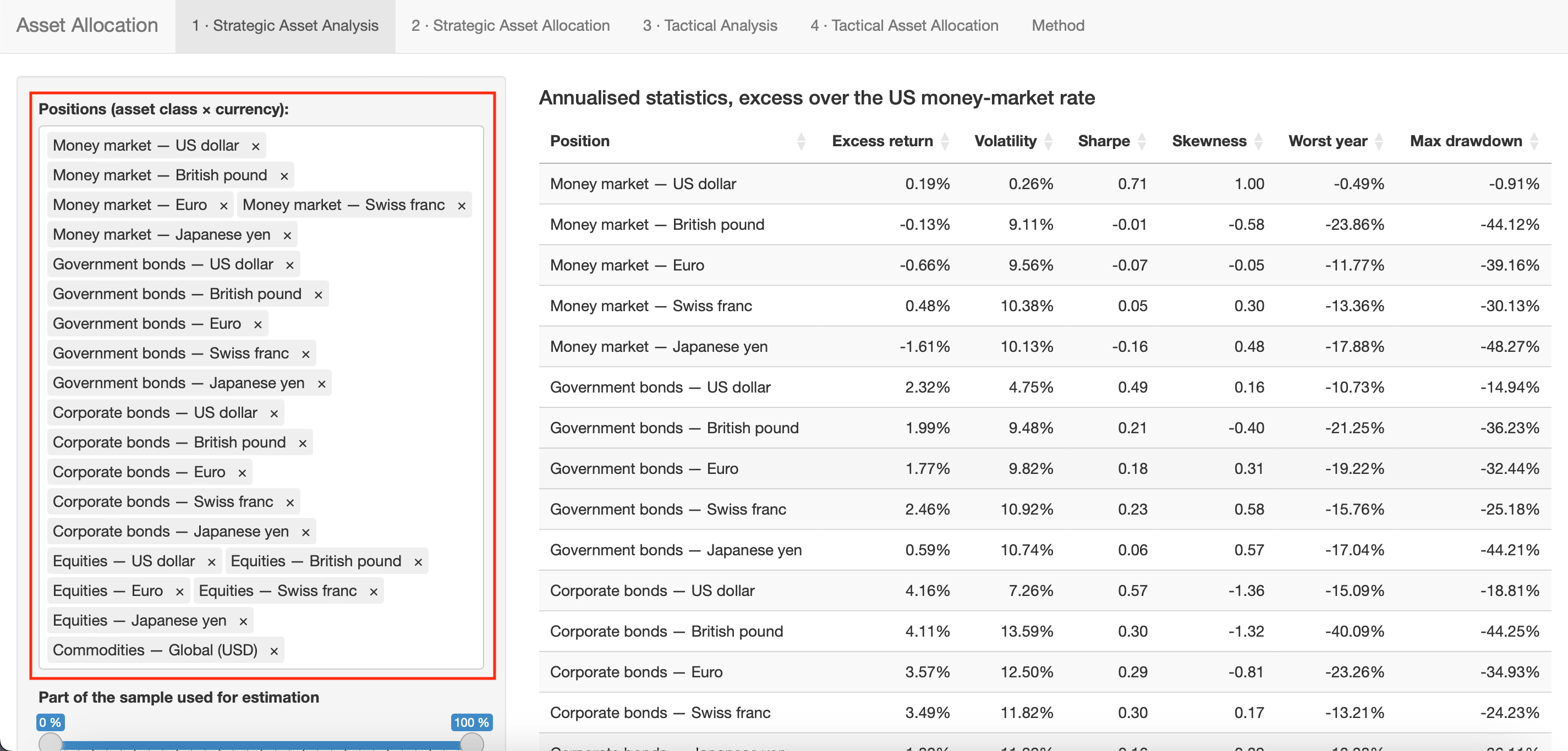
Select asset classes. In this screenshot the five money-market positions have been added to the default selection.

The five money-market positions are not part of the benchmark, so the default selection leaves them out. If you add them here, they also enter the optimisation in Station 2, and the allocation can then hold cash. Returns are in US dollars and unhedged, so a foreign money-market position carries almost the full volatility of its exchange rate.

A.2 Station 2: Strategic Asset Allocation

Based on the supplied inputs, Station 2 optimises the fund’s strategic allocation. This quadratic programme maximises the portfolio’s expected return while minimising its risk, subject to several constraints. As introduced in Chapter 4, the method follows the Markowitz mean–variance optimisation framework. Additional constraints account for the home market and home share, as well as floors and caps for asset classes, currencies, and individual positions.

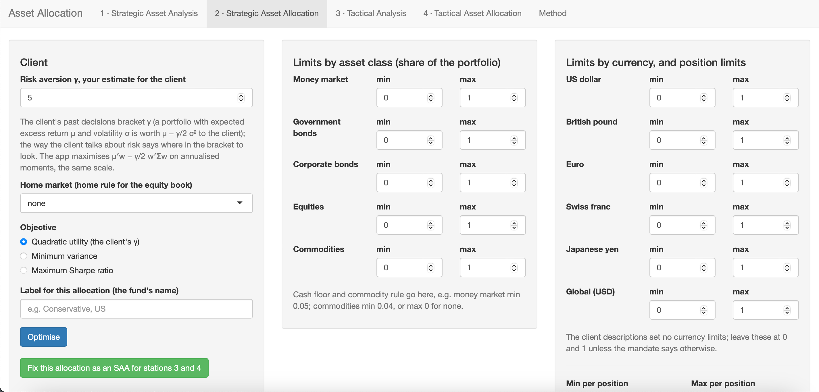
Set the parameters for the mean variance optimisation

For each fund, specify the risk-aversion parameter (γ), the home market, the home share, and the objective function: quadratic utility, minimum variance, or maximum Sharpe ratio. Optimal weights for each asset class and currency are then computed subject to the specified constraints.

With these inputs, the app solves the following optimisation problem:

\[ \max_w \; \mu' w - \frac{\gamma}{2}\, w' \Sigma w \quad \text{s.t.} \quad \sum w = 1,\; w \ge 0,\; \text{floors and caps},\; \text{home rule}, \]

with the home rule as one linear equality per foreign equity market: \(w_x = (1-h)\, s_x \sum_{\text{equity}} w\), where \(h\) is the home share and \(s_x\) the capitalisation share of the market \(x\) outside the home market.

A.3 Station 3: Tactical Analysis

Before calculating the tactical allocation, specify views on the expected returns of the assets. Views can be absolute or relative and can include a confidence level.

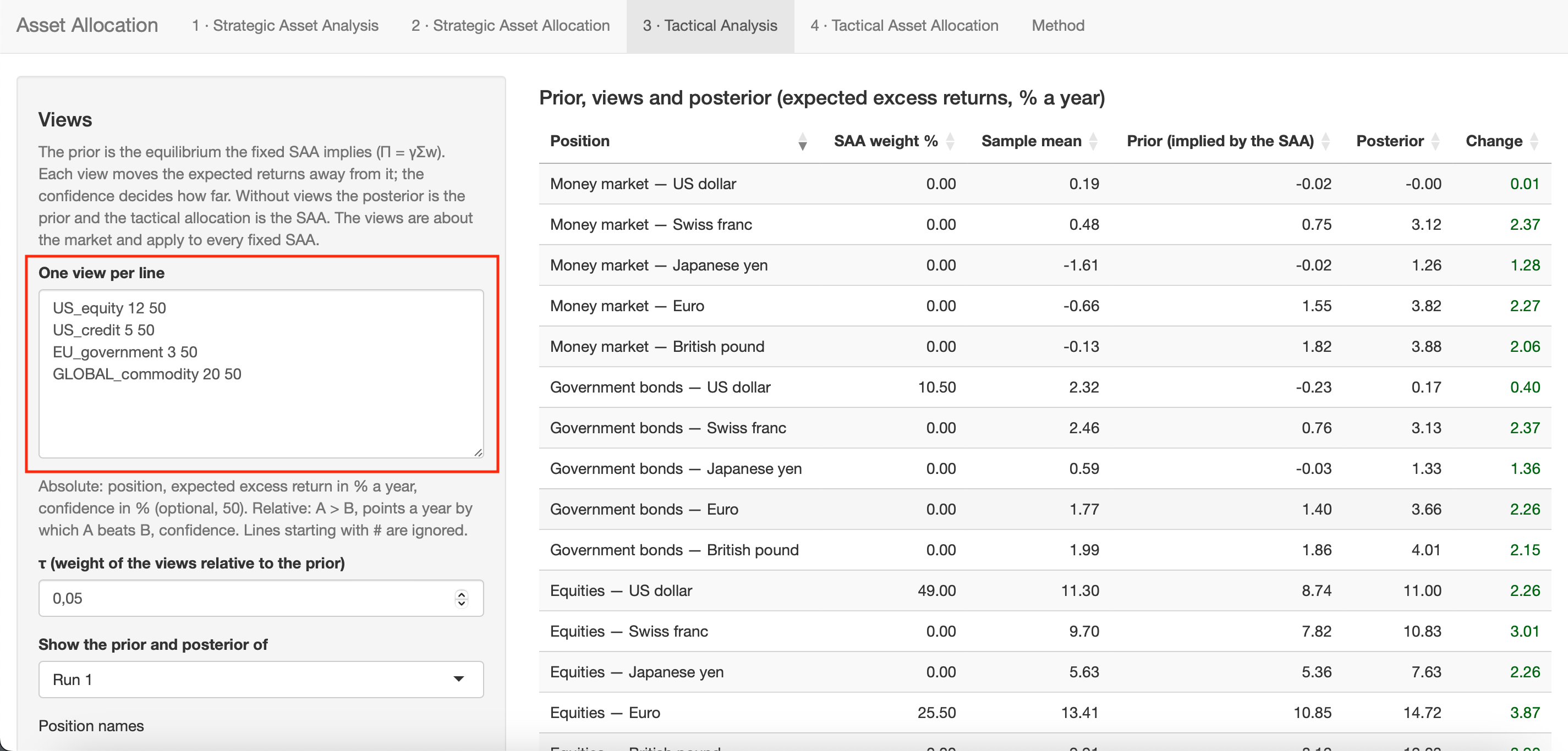
Use the following syntax for the views:

Positions are named <region>_<class>: US_money_market, UK_government, EU_credit, CH_equity, JP_equity, GLOBAL_commodity
- Money market: US_money_market, UK_money_market, EU_money_market, CH_money_market, JP_money_market
- Government bonds: US_government, UK_government, EU_government, CH_government, JP_government
- Corporate bonds: US_credit, UK_credit, EU_credit, CH_credit, JP_credit
- Equities: US_equity, UK_equity, EU_equity, CH_equity, JP_equity
- Alternatives: GLOBAL_commodity
Absolute view: <position> <expected return> [confidence] (e.g., US_equity 12 50 means that US equities are expected to earn 12% a year over cash, with a confidence of 50%)
Relative view: <position1> > <position2> <expected return difference> [confidence] (e.g., EU_equity > CH_equity 2 60 means that euro-area equities are expected to beat Swiss equities by 2 points a year, with a confidence of 60%)
Enter each view on a new line. Lines starting with # are ignored. A list of position names is available in the panel.

Parameter τ controls the weight assigned to the views during optimisation. Based on the specified views and strategic allocation, the app computes the prior and posterior expected returns.

These views produce the priors and posteriors through the He–Litterman (1999) model.

Prior — the baseline expected returns implied by the strategic allocation, before any tactical views. Reverse optimisation obtains it from \(\Pi = \gamma \Sigma w_{\text{SAA}}\): the SAA weights are treated as if they were optimal, and the returns that would justify them are backed out. The prior therefore anchors the analysis to the long-term allocation.
Posterior — the updated expected returns after incorporating the views. The Black–Litterman formula blends the prior (weighted by \(\tau\Sigma\), reflecting uncertainty in the prior) with the views \(Q\) (weighted by \(\Omega\), reflecting confidence in each view). High-confidence views move returns further from the prior; low-confidence views barely move them. In the positive-semidefinite sense, posterior covariance \(\Sigma_{BL}\) exceeds \(\Sigma\) because it adds estimation uncertainty to market risk.

A.4 Station 4: Tactical Asset Allocation

In the final step, translate the short-term views into a tactical allocation. Define the Strategic Asset Allocation (SAA) and the Tactical Analysis before computing the Tactical Asset Allocation (TAA). Solving an optimisation problem similar to the one in Station 2 produces the TAA, using the posterior expected returns and covariance matrix from Station 3, together with constraints on the maximum deviation per position and the tracking-error budget.

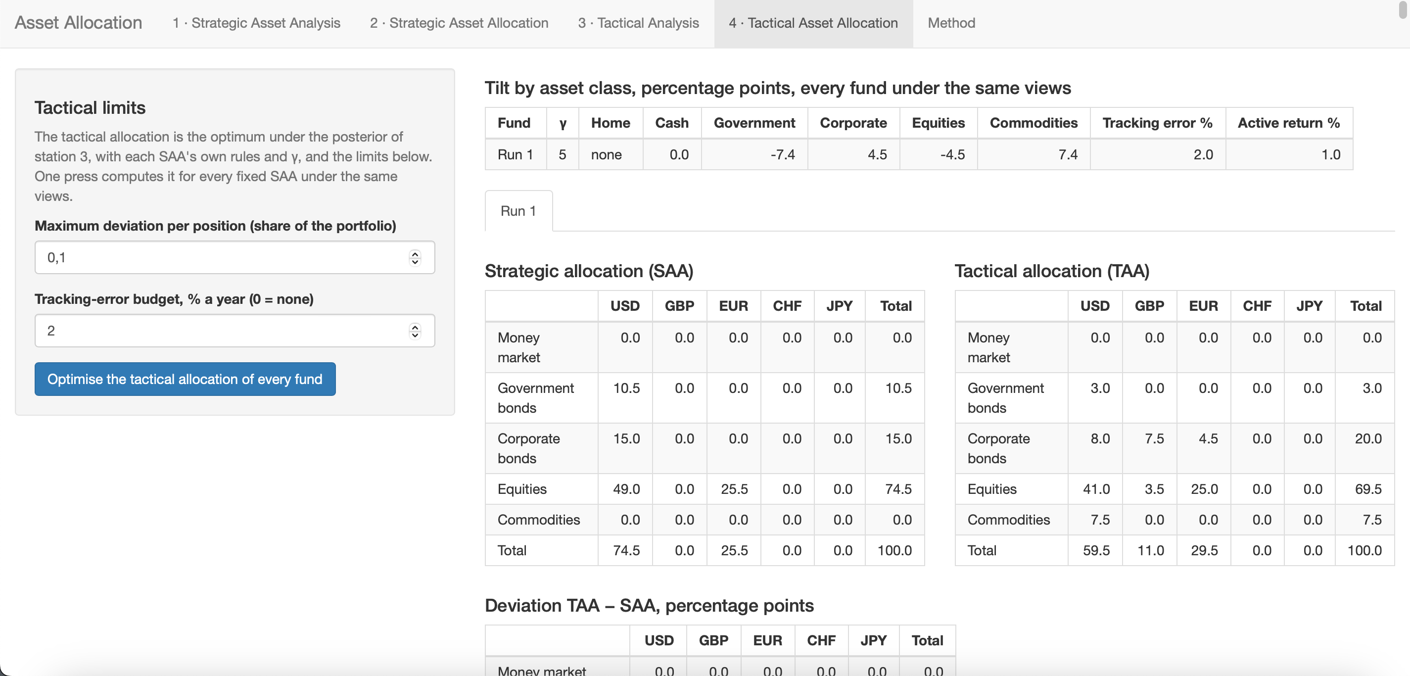
Optimise for the Tactical Asset Allocation

Specify the maximum deviation per position (the band; default: 0.05) and the tracking-error budget (default: 2% per year; 0 means no tracking-error constraint). Optimal weights for each asset class and currency are then computed subject to the specified constraints. This budget represents the maximum permitted deviation from the strategic allocation, measured as the standard deviation of the difference between the tactical and strategic allocations using the covariance matrix.

Station 4 drops the home rule. In Station 2 the rule fixes the split of the equity book across markets, so if it stayed in place, a view on an individual equity market could not change the allocation. Risk is measured with the sample covariance Σ rather than \(\Sigma_{BL}\); the latter adds estimation uncertainty and could shift weights independently of the views. If the tracking error \(\sqrt{(w - w_{\text{SAA}})'\Sigma(w - w_{\text{SAA}})}\) exceeds the budget, the deviation is scaled to the budget.