2 Reading the client
In professional investment management, building a portfolio is only one part of the process. Before deciding how to invest, the manager must understand the person the portfolio is being built for. Good investment management starts with the client’s needs.
2.1 What the Clients page gives you
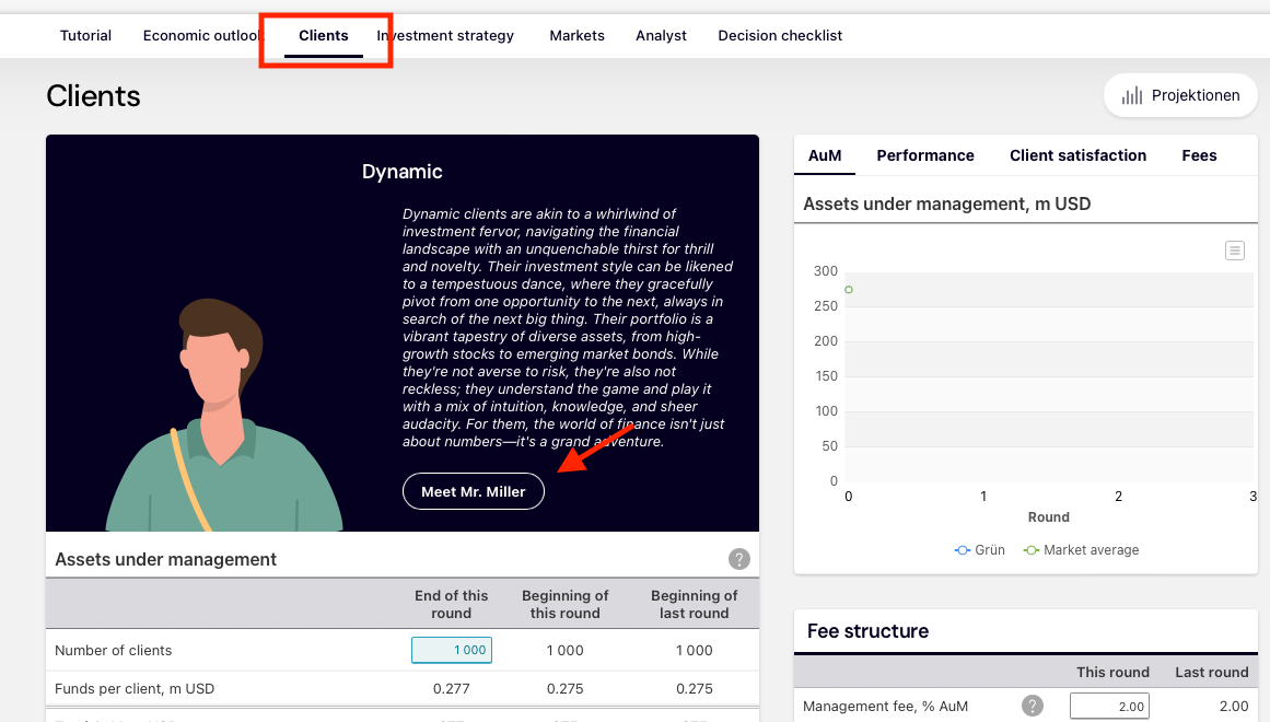
Each fund has a client card on the Clients page. It shows a general profile of the client type; the Meet client X button introduces a representative client.
The text contains everything the strategic allocation needs. In short, each client has one number and two rules:
- a risk aversion coefficient γ, which the text does not state as a number;
- a commodity rule (a minimum share, or none at all);
- a home rule: a share of the equity book in the client’s home market, the rest across the other markets in proportion to their size.
Some clients also have a sustainability requirement, and short sales are never allowed. Whatever the card does not mention is not constrained.
2.2 The rules: read them off
The rules are stated in plain words and mean exactly what they say. “They do not consider commodity futures compatible with their purpose” is a commodity cap of zero; “about five percent in commodities” is a floor of 5 %. “Half of the equities in companies from their home market, the rest spread across the other developed markets in proportion to their size” is the home rule with a home share of one half.
Write the rules down as numbers before you open the app. For the Hartley family, the invented client used throughout this book, the rules read:
Home market Britain. Commodities at least 5 %. Half of the equity book in UK companies, the rest by market size. No sustainability requirement. Cash at the manager’s discretion.
2.3 The risk aversion: bracket it from two decisions
The client card describes decisions the client has taken in the past. Each is a choice between two portfolios. For each portfolio the card gives two numbers: its volatility \(\sigma\) and its expected return over cash \(\mu\).
We need to turn those two decisions into a number, the client’s risk aversion \(\gamma\). The idea is simple. A risk-averse client dislikes volatility. Offered a portfolio with more return and more volatility and one with less of both, the client’s choice tells us roughly how much they dislike volatility. Two decisions give us two constraints, one on each side of the true \(\gamma\), and together they bracket it.
2.3.1 The utility function, in one line
To make “how much they dislike volatility” precise, we assume the client values a portfolio by its mean–variance utility:
\[ U = \mu - \frac{\gamma}{2}\sigma^2 \]
Read it as: utility = return minus a penalty for risk. The penalty is \(\frac{\gamma}{2}\) times the variance, so a client with a higher \(\gamma\) penalises risk more heavily. This is the standard Markowitz utility function, and the \(\gamma\) in it is the same risk aversion that appears in mean–variance optimisation in Chapter 4. Higher \(\gamma\) means a more cautious client.
A client prefers portfolio A to portfolio B when \(U_A > U_B\). Every past decision on the card is a statement of that form, and each one can be solved for \(\gamma\).
2.3.2 What one decision tells us
Take one decision. The client chose one portfolio over another. Call the one they chose the winner and the other the loser. We do not yet need to know which is riskier; write the winner’s return and volatility as \(\mu_W, \sigma_W\) and the loser’s as \(\mu_L, \sigma_L\).
The client preferred the winner, so its utility must be higher:
\[ \mu_W - \frac{\gamma}{2}\sigma_W^2 > \mu_L - \frac{\gamma}{2}\sigma_L^2 \]
Move the \(\gamma\) terms to the left and the return terms to the right:
\[ \frac{\gamma}{2}\left(\sigma_L^2 - \sigma_W^2\right) > \mu_L - \mu_W \]
Now look at the sign of \(\sigma_L^2 - \sigma_W^2\). It is positive if the loser was the riskier portfolio and negative if the winner was. That sign decides which way the inequality points, and therefore whether the decision gives us a floor or a ceiling on \(\gamma\).
Case 1: the client turned down the riskier portfolio. The winner is the quieter one, so the loser had the larger variance and \(\sigma_L^2 - \sigma_W^2 > 0\). Dividing by a positive number keeps the inequality pointing the same way:
\[ \gamma > \frac{2(\mu_L - \mu_W)}{\sigma_L^2 - \sigma_W^2} \]
The client gave up some return to get a quieter portfolio. That means they must be at least this risk-averse. The decision gives us a floor on \(\gamma\).
Case 2: the client took the riskier portfolio. The winner is the riskier one, so the loser had the smaller variance and \(\sigma_L^2 - \sigma_W^2 < 0\). Dividing by a negative number flips the inequality:
\[ \gamma < \frac{2(\mu_W - \mu_L)}{\sigma_W^2 - \sigma_L^2} \]
The client was willing to accept more swing to get more return. That means they cannot be more risk-averse than this. The decision gives us a ceiling on \(\gamma\).
2.3.3 The one formula to remember
Notice that the right-hand side is the same expression in both cases, once you put the riskier portfolio on top. Write \(X\) for the riskier portfolio and \(Y\) for the quieter one. Then:
\[ \text{bound} = \frac{2(\mu_X - \mu_Y)}{\sigma_X^2 - \sigma_Y^2} \]
and the only question is whether it is a floor or a ceiling:
- If the client rejected the riskier portfolio \(X\), the bound is a floor: \(\gamma > \text{bound}\).
- If the client chose the riskier portfolio \(X\), the bound is a ceiling: \(\gamma < \text{bound}\).
That is the whole method. You do not need to remember two formulas. You need to remember one expression and one question: which portfolio did the client end up with? If they ended up with the quieter one, the expression is a floor. If they ended up with the riskier one, it is a ceiling.
2.3.4 Two conditions for the bound to mean anything
The method only works if the two portfolios are genuinely different in both dimensions.
- The riskier portfolio must also offer more return. If the riskier portfolio offered less return, no sensible client would hold it, and the choice would tell us nothing about \(\gamma\). Always check that \(\mu_X > \mu_Y\) before applying the formula.
- Both numbers must be in the same units. Put \(\mu\) and \(\sigma\) in the same units (both decimals, both annualised). The \(\gamma\) you recover is then on the same scale as the \(\gamma\) that goes into the mean–variance optimiser in Chapter 4.
If either condition fails, the decision is not usable and you should look for another one on the card.
2.3.5 Worked example: the Hartleys
Decision 1: they turned down the riskier portfolio. With their previous adviser they rejected a portfolio with 10 % volatility and 6.9 % expected return over cash, and took one with 8 % volatility and 5.9 % instead. Here \(X=(10\%,\,6.9\%),\ Y=(8\%,\,5.9\%)\), and because they rejected \(X\) this is a lower bound:
\[ \gamma > \frac{2(0.069-0.059)}{0.10^2-0.08^2}=\frac{0.020}{0.0036}=5.6 \]
Decision 2: they kept the riskier portfolio. Later, offered an alternative with 6 % volatility and 5.1 % expected return over cash, they stayed with their portfolio of 8 % volatility and 6.6 %. Here \(X=(8\%,\,6.6\%),\ Y=(6\%,\,5.1\%)\), and because they chose \(X\) this is an upper bound:
\[ \gamma < \frac{2(0.066-0.051)}{0.08^2-0.06^2}=\frac{0.030}{0.0028}=10.7 \]
So the two decisions bracket the Hartleys:
\[ 5.6 < \gamma < 10.7 \]
that is, \(\gamma\) lies between about 5.5 and 11.
Placing \(\gamma\) inside the bracket. The bracket comes from what the client did; the words on the card place \(\gamma\) within it:
- “Lived through two bear markets without selling, but would not want to see a year like the worst they have lived through again” → middle of the bracket.
- “They need the portfolio to grow; income covers spending” → lower end (growth first, more tolerant of risk).
- “The income the portfolio produces matters more than growth” → higher end (capital preservation, less tolerant of risk).
For the Hartleys the bear-market comment points to the middle, so we take \(\gamma=8\).
2.4 From γ to a portfolio
Once \(\gamma\) is estimated, it does two things in the rest of the book. It selects the strategic allocation in Chapter 4, and it sets the prior of the Black–Litterman step in Chapters 5 and 6.
In Chapter 4, the client’s \(\gamma\) selects the point on the efficient frontier that maximises \(U=\mu-\frac{\gamma}{2}\sigma^2\). A higher \(\gamma\) selects a portfolio with less variance and a lower expected return; a lower \(\gamma\) selects a riskier one with a higher expected return. Do not read γ off a conventional profile table (“above 6 is conservative”): which equity share a γ produces depends on the data and the client’s rules. The Hartleys, at γ = 8, hold 46.5 % equities; the check is the guidance bands below, not a rule of thumb.
The rules are the same for every reader of the card. What distinguishes a careful reading from a careless one is the estimate of \(\gamma\). Chapter 4 shows what it costs to be wrong: for the Hartleys, \(\gamma = 7\) or \(9\) instead of \(8\) puts the allocation 7 or 5.5 points away from the benchmark; the ends of the bracket cost 14 to 23 points.
2.5 The guidance bands
Guidance bands are quoted in the text (“between 15 and 52 percent in government bonds”). They are the range inside which the client expects to be held, and they are consistent with the client’s risk aversion: every γ in the bracket gives an allocation inside the bands, and a γ outside the bracket leaves at least one band. Use them two ways: as a check on your allocation, and to narrow the bracket. If your allocation leaves a band, your γ is outside the bracket.
A fund held far from what the card describes loses the client, whatever the market does; a dynamic client parked in money market walks away. Lost clients mean lower AuM and lower profit, and in the end put the firm in financial difficulty.
2.6 The home market
Meet client X names the home market. It decides which equity market carries the home share of the equity book; the rest of the book goes to the other markets by capitalization (US 70.0, euro area 14.5, Japan 5.9, Switzerland 5.7, Britain 4.0 percent of the universe, renormalized without the home market). Because the home rule puts a large part of the equities into a market the data might not otherwise hold at that size, the rest of the allocation adjusts around it: two clients with the same γ and different home markets do not hold the same class mix. That is the method working, not a mistake.
2.6.1 Why the rest goes by size
The home share is the client’s own choice: most investors hold more of their home market than its size alone would justify, the well-documented home bias (French and Poterba 1991). For the rest of the equity book the client states no view, and the allocation should not invent one. Market capitalization is the weighting that needs no forecast. It is the market portfolio of the CAPM (Sharpe 1964), the one portfolio all investors can hold together, so any other weighting is a bet against the average investor (Sharpe 1991). It also protects the allocation from the optimizer: the expected returns of the five equity markets are estimated with an error larger than the differences between them, and a free optimization turns that noise into extreme weights, often a whole market at zero (Michaud 1989). Fixing the regional split by size leaves γ as the one number the reading of the card has to get right. And it keeps the strategic allocation consistent with Chapters 5 and 6, which reverse-optimize it into the prior of the Black–Litterman step: with the regions at market weights, that prior is close to the market equilibrium Black and Litterman start from (Black and Litterman 1992). The price of the rule is concentration. The United States is 70 percent of the universe, and capitalization weights follow a market into its bubbles, as Japan’s share of world equity around 1989 showed.
2.7 Sustainability
A client who requires a minimum rating holds only securities that pass it. This binds when tactical weights become positions (Chapter 7), not at the strategic level: the class-level statistics of the market do not change with the filter.
2.8 Deliverable of this step
Before the next step, write down what defines the client: γ with its bracket, the commodity rule, the home market and home share, and any sustainability requirement.
That gives one line per fund, which the next steps build on.
For the Hartleys:
Hartley, home UK: γ ≈ 8 (bracket 5.5–11), commodities ≥ 5 %, half of equities in the UK, no sustainability floor, cash at the manager’s discretion.
That line is the complete input to the strategic allocation.