Validating the event-clock estimator • eventclock

library(eventclock)

This vignette stress-tests the estimator $\widehat A = \sum (\Delta L)^2$ against data simulated from the exact transition law of the model (ec_simulate_path()), so every deviation is attributable to the estimator, not to model error. Helper to turn simulated paths into event_prices:

path_to_ep <- function(p) {
  as_event_prices(
    tibble::tibble(time = as.Date("2020-01-01") + p$step, q = p$q),
    clip = c(1e-8, 1 - 1e-8)
  )
}

estimate_A <- function(n_steps, A, q = 0.4, reps = 200, ...) {
  vapply(seq_len(reps), function(i) {
    p <- ec_simulate_path(1, n_steps, q = q, A = A, ...)
    event_clock(path_to_ep(p), methods = "rv")$A
  }, numeric(1))
}

Consistency and finite-sample precision

The estimator is unbiased at every sampling frequency (up to the tiny $\sum a_i^2/4$ drift term) and its dispersion shrinks with the number of observations:

grid <- c(15, 30, 60, 120, 250)
sims <- lapply(grid, estimate_A, A = 0.5)
tab <- data.frame(
  n_obs = grid,
  mean = sapply(sims, mean),
  bias_pct = 100 * (sapply(sims, mean) / 0.5 - 1),
  sd = sapply(sims, sd),
  rmse = sapply(sims, function(s) sqrt(mean((s - 0.5)^2)))
)
knitr::kable(tab, digits = 3)

n_obs	mean	bias_pct	sd	rmse
15	0.520	3.986	0.202	0.203
30	0.522	4.468	0.132	0.134
60	0.505	0.964	0.088	0.088
120	0.502	0.427	0.070	0.070
250	0.501	0.289	0.043	0.043

Even the paper-sized windows (a one-month window has about 30 daily observations) are unbiased; the price of short windows is dispersion, not bias — which is why interval estimates matter.

Confidence-interval coverage

event_clock(se = TRUE) reports quarticity-based standard errors with log-scale intervals. Their coverage is close to nominal:

coverage <- function(conf, reps = 300, n_steps = 60, A = 0.5) {
  hits <- vapply(seq_len(reps), function(i) {
    p <- ec_simulate_path(1, n_steps, q = 0.4, A = A)
    r <- event_clock(path_to_ep(p), methods = "rv", se = TRUE, conf = conf)
    r$ci_lo <= A && A <= r$ci_hi
  }, logical(1))
  mean(hits)
}
data.frame(
  nominal = c(0.90, 0.95),
  empirical = c(coverage(0.90), coverage(0.95))
)
#>   nominal empirical
#> 1    0.90 0.8833333
#> 2    0.95 0.9500000

Outcome independence: the measure-robustness property in action

Quadratic variation does not care which outcome eventually realizes — this is the observable footprint of measure robustness (a change of measure reweights outcomes; it cannot change the estimate computed from a given path):

p <- ec_simulate_path(400, 60, q = 0.4, A = 0.5)
qv <- vapply(split(p$L, p$path), function(L) sum(diff(L)^2), numeric(1))
J <- vapply(split(p$J, p$path), function(j) j[1], numeric(1))
data.frame(
  outcome = c("J = 1", "J = 0"),
  mean_A_hat = c(mean(qv[J == 1]), mean(qv[J == 0])),
  n_paths = c(sum(J == 1), sum(J == 0))
)
#>   outcome mean_A_hat n_paths
#> 1   J = 1  0.4935467     169
#> 2   J = 0  0.5079064     231

Both conditional means sit at the same true $A = 0.5$ : the clock measures how much was learned, not what was learned.

Lumpy information: what the robustness variants actually do

Real event clocks are lumpy — debates and verdicts, not a smooth flow. With jump_share, the simulator concentrates part of $A$ in a few jump steps, and the estimator battery reacts exactly as the theory says it should:

lumpy <- lapply(seq_len(200), function(i) {
  p <- ec_simulate_path(1, 60, q = 0.4, A = 0.5,
                        jump_share = 0.5, n_jumps = 1)
  event_clock(path_to_ep(p))[, c("method", "A")]
})
agg <- do.call(rbind, lumpy)
knitr::kable(
  aggregate(A ~ method, data = agg, FUN = mean),
  digits = 3,
  caption = "Mean estimate across 200 lumpy paths (true A = 0.5, half of it in one jump)"
)

Mean estimate across 200 lumpy paths (true A = 0.5, half of it in one jump)
method	A
bipower	0.301
largest1	0.240
largest2	0.214
rv	0.502
truncated	0.236

rv recovers total clock time including the jump; bipower, truncated, and largest1 estimate (roughly) the smooth component only — the gap between rv and bipower is the jumpiness index. None of these is “wrong”; they answer different questions, and comparing them is the point.

Microstructure noise and the snapshot rule

Traded quotes bounce between bid and ask on a coarse tick grid. Additive noise inflates measured variation at fine sampling — the classic signature-plot diagnostic, here on simulated data with known truth:

p <- ec_simulate_path(1, 2000, q = 0.4, A = 1)
noisy <- ec_ilogit(p$L + rnorm(nrow(p), sd = 0.04))
ep_noisy <- as_event_prices(
  tibble::tibble(time = as.POSIXct("2024-01-01", tz = "UTC") +
                   3600 * p$step, q = noisy),
  clip = c(1e-8, 1 - 1e-8)
)
plot_signature(ec_signature(ep_noisy, max_every = 24))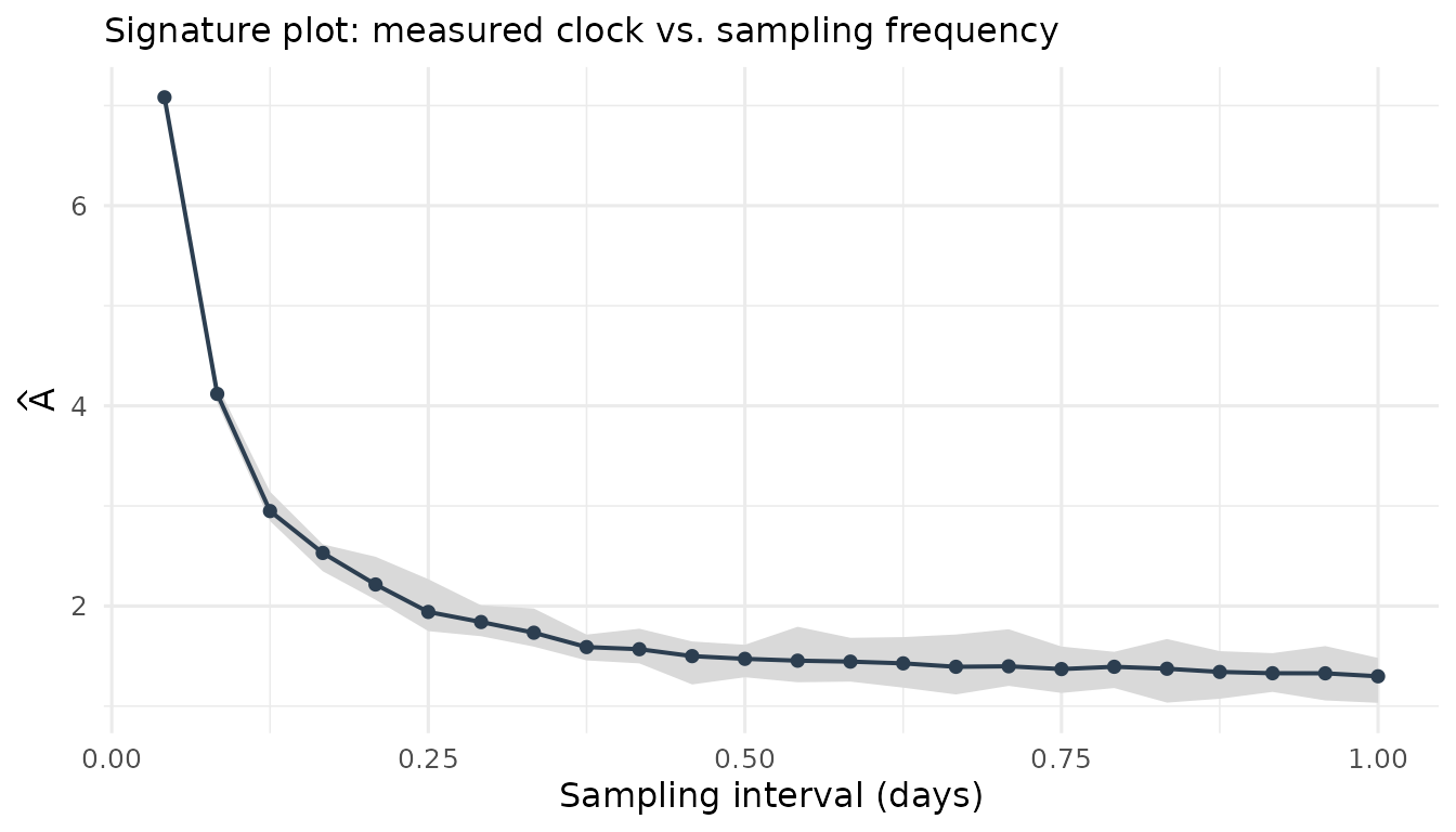

The finest grid overstates the clock (noise variance is counted once per increment); sparse sampling converges toward the true $A = 1$ . On real data the same pattern appears — this is the hourly-vs-daily gap of the 2024 Polymarket series:

data(polymarket2024)
plot_signature(ec_signature(as_event_prices(polymarket2024), max_every = 24))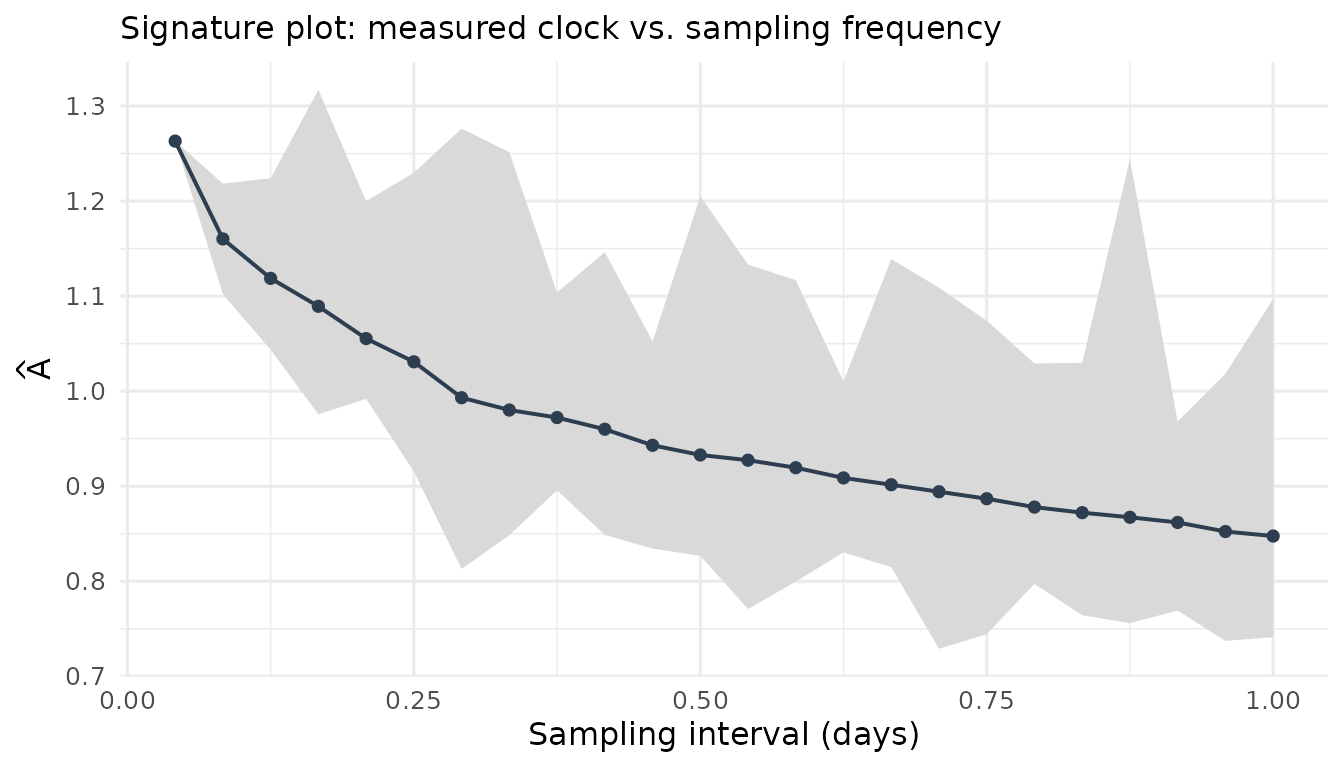

which is why the one-snapshot-per-day rule of pm_daily() is the robust default for daily-horizon work.

Data-quality screening

Before estimating anything, screen the input series:

ec_validate(as_event_prices(brexit2016, time = "date", price = "q_leave",
                            market_id = "Brexit: Leave"))
#> -- Event-price data-quality report: Brexit: Leave
#> Coverage:  119 obs, 2016-02-26 to 2016-06-23, median spacing 1 days, 0 NA
#> Clipping:  0.0% of observations outside the clipping bounds
#> Staleness: 11.0% zero increments, longest stale run 2 obs
#> Tick:      smallest non-zero move 0.001
#> Gaps:      0 gap increment(s), largest 1 days
#> Outliers:  max |dL| = 0.292 (5.5 robust SDs)

ec_validate() reports coverage, staleness, tick size, gaps, and outliers — in the package’s flag-don’t-drop spirit: nothing is altered, everything is visible.