Event-spanning options: estimating the event exposure • eventclock

library(eventclock)

Two kinds of options around a scheduled event

An option that expires after a scheduled event is exposed to the realized outcome itself: its price depends on how the asset is distributed conditional on each outcome. An option that expires before resolution is exposed only to learning — revisions in the event probability while the option is alive. The working paper’s sequential design keeps these roles strictly separate:

the traded event market supplies the state-price-implied event probability $q_t$ and, via the event clock, the information-flow input (q_from_price(), event_clock());
event-spanning options identify the outcome-conditional asset distributions — this vignette;
pre-resolution options and the underlying are held out and used as overidentifying restrictions, not as calibration instruments.

This vignette covers step 2: the lognormal event mixture, the event exposure $\theta \;=\; \log\!\big(m_1 / m_2\big),$ the log ratio of the outcome-conditional risk-neutral means of the event multiplier, and how to estimate a common $\theta$ from a panel of event-spanning option surfaces.

The lognormal event mixture

Normalize the terminal asset value by its forward. Conditional on outcome 1 (probability $q$ ) the gross event multiplier is lognormal with conditional mean $m_1$ and total dispersion $s_1$ ; conditional on outcome 2 it is lognormal with mean $m_2$ and dispersion $s_2$ . The pricing-measure adding-up (scale) normalization $q\,m_1 + (1-q)\,m_2 \;=\; 1$ fixes the level, so $(q, \theta, s_1, s_2)$ fully parametrize the mixture. ec_mix_price() prices forward-normalized European options; ec_mix_iv() converts them into Black implied dispersions:

k <- seq(-0.6, 0.6, by = 0.04)
smile <- function(theta) ec_mix_iv(k, q = 0.35, theta = theta,
                                   s1 = 0.25, s2 = 0.25)
dat <- data.frame(
  k = rep(k, 3),
  iv = c(smile(0), smile(0.5), smile(1.0)),
  theta = factor(rep(c("theta = 0", "theta = 0.5", "theta = 1.0"),
                     each = length(k)))
)
library(ggplot2)
ggplot(dat, aes(k, iv, colour = theta)) +
  geom_line(linewidth = 0.8) +
  labs(x = "log-forward moneyness k", y = "total implied dispersion",
       colour = NULL) +
  theme_minimal()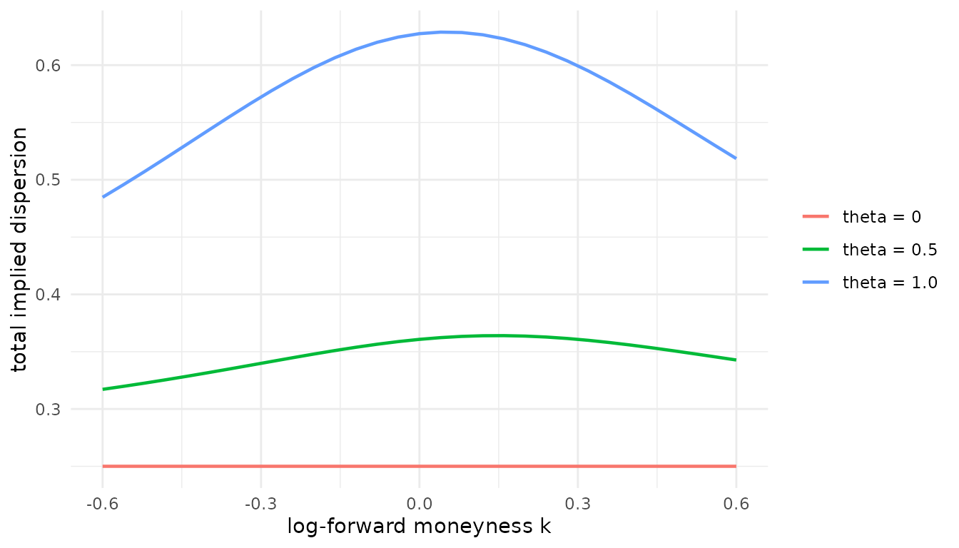

Implied-dispersion smiles of the event mixture for increasing event exposure

With $\theta = 0$ the mixture collapses to a single lognormal and the smile is flat. A nonzero exposure adds the two-point outcome spread on top of the conditional dispersions: the smile rises and, away from $q = 1/2$ , becomes asymmetric. That asymmetry is exactly what the surface fit uses.

Two useful identities connect this family to the rest of the package:

to first order, $\theta$ is the event beta. The returns-based exposure of event_beta() estimates $\Delta\eta = \eta_1 - \eta_2$ , and for small exposures $\Delta\eta \approx \theta$ : the two measurements are the same object seen from returns and from option smiles;
the event contributes $q(1-q)\,\theta^2$ of total log variance (exactly, when the conditional dispersions coincide) — the basis of the quick estimator below.

Delta grids

Standardized option surfaces are usually delivered on a (call-equivalent) delta grid rather than in strikes. ec_delta_to_k() maps the grid into log-forward moneyness, node by node, using the node’s own total dispersion — so no forward reconstruction is needed:

iv <- c(0.32, 0.29, 0.27, 0.26, 0.27)   # annualized, 30 days to expiry
tau <- 30 / 365
node <- c(0.1, 0.3, 0.5, 0.7, 0.9)
ec_delta_to_k(node, s = iv * sqrt(tau))
#> [1]  0.12177923  0.04705504  0.00299589 -0.03631057 -0.09620465

Put deltas enter as call-equivalent deltas, $\Delta = 1 + \delta_{put}$ , so a standard OTM composite smile (calls below 0.5, puts above) becomes one monotone grid.

Estimating a common exposure from spanning surfaces

The working paper’s design gives every surface (one valuation date, one event-spanning expiry) its own conditional dispersions, while the exposure $\theta$ is restricted to be common across all surfaces; the objective is surface balanced, so each surface counts equally. ec_theta_fit() implements exactly this. Here we simulate a small clean panel with a known $\theta = 0.8$ and recover it:

k7 <- seq(-0.5, 0.5, length.out = 7)
cfg <- data.frame(
  surface = c("oct25_nov15", "oct28_nov15", "nov01_nov22"),
  q  = c(0.40, 0.45, 0.42),
  s1 = c(0.28, 0.27, 0.30),
  s2 = c(0.35, 0.33, 0.38)
)
panel <- do.call(rbind, lapply(seq_len(nrow(cfg)), function(i) {
  data.frame(
    surface = cfg$surface[i], k = k7, q = cfg$q[i],
    iv = ec_mix_iv(k7, cfg$q[i], theta = 0.8, cfg$s1[i], cfg$s2[i])
  )
}))
fit <- ec_theta_fit(panel)
fit
#> -- Event-spanning mixture fit (3 surfaces, 21 nodes)
#> Common event exposure theta = 0.8000 (conditional-mean ratio m1/m2 = 2.226)
#> Surface-balanced RMSE = 0.0000 (IV units of the input)

The per-surface table reports the fitted conditional dispersions and per-surface fit quality:

fit$surfaces
#> # A tibble: 3 × 7
#>   surface         q     n theta    s1    s2       rmse
#>   <chr>       <dbl> <int> <dbl> <dbl> <dbl>      <dbl>
#> 1 oct25_nov15  0.4      7 0.800 0.280 0.350 0.00000176
#> 2 oct28_nov15  0.45     7 0.800 0.270 0.330 0.00000248
#> 3 nov01_nov22  0.42     7 0.800 0.300 0.380 0.00000156

Supply annualized IVs together with a tau column (years to expiry) to work in annualized units, and a w column (for instance the number of quotes behind each node) to weight nodes within a surface.

common = FALSE is the free-ratio diagnostic: every surface picks its own $\theta$ , and the comparison with the common fit shows how much the cross-surface restriction costs — in the working paper’s 2024 application the deterioration is modest while the common ratio is stable across maturities, which is what makes the exposure credible.

Sign identification. At $q = 1/2$ the mixture is observationally symmetric in $(\theta, s_1, s_2) \mapsto (-\theta, s_2, s_1)$ : option prices alone cannot say which outcome the asset favors. When $q$ is close to one half, fix the sign externally — the returns-based event_beta() against the same event-probability series is the natural source.

The quick estimator: the variance hump

Often an existing pipeline already computes a maturity hump — how much higher the event-spanning expiry’s volatility is than its neighbors’. Worked in total variance units (not annualized volatilities), that hump is the event’s variance contribution $q(1-q)\,\theta^2$ , and ec_theta_hump() inverts it:

tau_b <- 35 / 365
iv_spanning <- 0.21   # event-spanning ATM, annualized
iv_baseline <- 0.15   # no-event baseline at the same maturity
dvar <- (iv_spanning^2 - iv_baseline^2) * tau_b
ec_theta_hump(dvar, q = 0.4)
#> [1] 0.09289853

This is a first-order magnitude estimate — it needs no optimization and no wing data, which makes it the natural first pass over a large cross-section before running the full surface fit on the assets that matter. It identifies $|\theta|$ only; the sign again comes from event_beta().

Clock sensitivity: partial recovery

The spanning estimation uses only the level $q_t$ . As soon as the estimated exposure feeds a pre-resolution learning exercise, the event clock enters, and the measured log-odds variation identifies the physical clock only under the exact-recovery restriction. The working paper’s sensitivity grid replaces the point clock with the sharp partial-recovery interval, which ec_recovery_set() tabulates:

ec_recovery_set(0.511)   # the Brexit one-month clock
#> # A tibble: 4 × 4
#>       A   eps lower upper
#>   <dbl> <dbl> <dbl> <dbl>
#> 1 0.511  0    0.511 0.511
#> 2 0.511  0.1  0.414 0.618
#> 3 0.511  0.25 0.287 0.798
#> 4 0.511  0.5  0.128 1.15

At eps = 0 (exact recovery) the interval degenerates to the measured value; wider bounds propagate economically motivated uncertainty about state-dependent valuation into everything downstream.

What this vignette did not do

The package deliberately ships no proprietary option data: the estimation functions take your surfaces in the long format shown above. The full sequential design — counterfactual shape from post-resolution surfaces, held-out pre-resolution wing tests, and dependence between ordinary asset news and event-probability innovations — lives in the accompanying working paper (Hanke, Schadner, Stöckl, and Weissensteiner, Working Paper, “Learning Before Scheduled Events: Prediction Markets, State Prices, and Option Valuation”); the transition machinery needed to price pre-resolution claims under learning is already available via ec_transition_density(), ec_simulate(), and the formula-book calculators (ec_atm_event_call(), ec_iv_rule()).