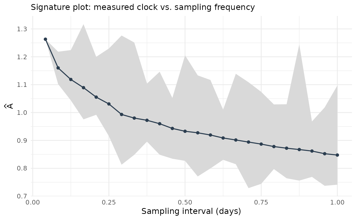
Computes the clock estimate \(\widehat A\) across sampling frequencies — the analogue of the volatility signature plot. For each subsampling step \(k\), the realized variation is averaged over all \(k\) possible offsets of the sparse grid. A pronounced increase of \(\widehat A\) at the finest frequencies signals microstructure noise (bid-ask bounce on a coarse tick grid); a flat signature means the clock is measured cleanly.
Usage
ec_signature(x, max_every = 10, from = NULL, to = NULL, clip = NULL)

# S3 method for class 'ec_signature'
plot(x, ...)
Arguments
- x
An
event_pricesobject (seeas_event_prices()), or adata.framecoercible to one.- max_every
Integer, largest subsampling step (default 10).
- from
Valuation date/time (default: first observation).
- to
One or more horizon dates/times (default: last observation = full sample). Names are used as horizon labels.
- clip
Numeric length-2 clipping bounds for
qbefore the log-odds transform; defaults to the bounds stored inx.- ...
Unused (for the
plotmethod).
Value
A tibble of class ec_signature with columns
- sample_every
subsampling step \(k\).
- spacing_days
median spacing of the sparse grid in days.
- n_incr
average number of increments per offset grid.
- A
realized variation averaged over the \(k\) offsets.
- A_min, A_max
range over the offsets.
Methods (by generic)
plot(ec_signature): Plot method; dispatches toplot_signature().
Examples
data(polymarket2024)
sig <- ec_signature(as_event_prices(polymarket2024), max_every = 24)
head(sig)
#> # A tibble: 6 × 6
#>   sample_every spacing_days n_incr     A A_min A_max
#>          <int>        <dbl>  <dbl> <dbl> <dbl> <dbl>
#> 1            1       0.0417  3790   1.26 1.26   1.26
#> 2            2       0.0833  1894.  1.16 1.10   1.22
#> 3            3       0.125   1263.  1.12 1.04   1.22
#> 4            4       0.167    947.  1.09 0.976  1.32
#> 5            5       0.208    757.  1.06 0.992  1.20
#> 6            6       0.25     631.  1.03 0.915  1.23
plot_signature(sig)