
2. Post-processing forecasts: correcting the moments you were handed
Source:vignettes/rafe-post-processing.Rmd
rafe-post-processing.Rmdvignette("rafe-evaluation", package = "rafe") showed
that the Sharpe gap of a plug-in portfolio is bounded by two channels: a
mean error measured in the risk metric (RAFE) and a covariance
distortion measured in the operator norm (C-RAFE). This vignette does
something about them.
The premise is that you have already been handed — from a sample estimate, a vendor model, a machine-learning pipeline — and you cannot retrain it. What you can do is correct the moments before they reach the optimiser. That is the subject of the moment-correction working paper cited below.
The two atomic correctors
mu_rafe_stein() shrinks the mean toward a target with
intensity
,
computing that intensity in the
-whitened
space. Pass T_obs for the positive-part James-Stein
intensity implied by the sample size:
window    <- R[1:60, ]
mu_hat    <- colMeans(window)
Sigma_hat <- stats::cov(window)

mu_js <- mu_rafe_stein(mu_hat, Sigma_hat, T_obs = 60)
attr(mu_js, "kappa")
#> [1] 0.3704

round(rbind(raw = mu_hat, corrected = as.numeric(mu_js)), 4)[, 1:6]
#>            NoDur  Durbl  Manuf  Enrgy  Chems  BusEq
#> raw       0.0083 0.0042 0.0098 0.0078 0.0024 0.0124
#> corrected 0.0078 0.0053 0.0088 0.0075 0.0041 0.0104
The corrector pulls the cross-section toward its own grand mean while leaving that grand mean untouched:
c(raw = mean(mu_hat), corrected = mean(mu_js),
  raw_spread = sd(mu_hat), corrected_spread = sd(mu_js))
#>              raw        corrected       raw_spread corrected_spread
#>         0.007029         0.007029         0.004908         0.003090
sigma_crafe_floor() lifts the small eigenvalues of
to a floor set relative to the mean eigenvalue. Those small eigenvalues
are exactly the directions a mean-variance optimiser leverages hardest,
and exactly where the sample covariance is least trustworthy:
lam_raw <- eigen(Sigma_hat, symmetric = TRUE)$values
lam_cln <- eigen(sigma_crafe_floor(Sigma_hat, 0.3), symmetric = TRUE)$values
round(rbind(raw = lam_raw, floored = lam_cln), 5)
#>            [,1]    [,2]  [,3]    [,4]  [,5]    [,6]    [,7]    [,8]    [,9]
#> raw     0.01264 0.00166 0.001 0.00071 6e-04 0.00039 0.00033 0.00027 0.00022
#> floored 0.01264 0.00166 0.001 0.00071 6e-04 0.00045 0.00045 0.00045 0.00045
#>           [,10]   [,11]   [,12]
#> raw     0.00018 0.00009 0.00005
#> floored 0.00045 0.00045 0.00045
c(condition_raw = max(lam_raw) / min(lam_raw),
  condition_floored = max(lam_cln) / min(lam_cln))
#>     condition_raw condition_floored
#>            262.58             27.87
Choosing and from data
Neither intensity should be picked by hand. Both tuners split the training window into an inner-training and an inner-validation block (40 + 20 months by default), fit on the first and score on the second.
They differ in what they score. sep_tune()
tunes each parameter against its own channel —
on inner-validation RAFE,
on inner-validation C-RAFE. joint_trafe_tune() searches the
full
grid against inner-validation T-RAFE.
kg <- seq(0, 1, by = 0.05)
tg <- seq(0, 0.5, by = 0.05)

fit_sep   <- sep_tune(window, kappa_grid = kg, tau_grid = tg)
fit_joint <- joint_trafe_tune(window, kappa_grid = kg, tau_grid = tg)

rbind(sep   = c(kappa = fit_sep$kappa,   tau = fit_sep$tau_rel),
      joint = c(kappa = fit_joint$kappa, tau = fit_joint$tau_rel))
#>       kappa tau
#> sep       1 0.5
#> joint     1 0.5
sep_tune() returns the two loss profiles, so you can see
whether the optimum is interior or sitting on a grid edge:
op <- par(mfrow = c(1, 2), mar = c(4.2, 4.2, 2.4, 1))
plot(kg, fit_sep$losses_kappa, type = "l", lwd = 2, col = "steelblue",
     xlab = expression(kappa), ylab = "inner-validation RAFE",
     main = "Mean channel")
abline(v = fit_sep$kappa, lty = 2)
plot(tg, fit_sep$losses_tau, type = "l", lwd = 2, col = "darkorange",
     xlab = expression(tau), ylab = "inner-validation C-RAFE",
     main = "Covariance channel")
abline(v = fit_sep$tau_rel, lty = 2)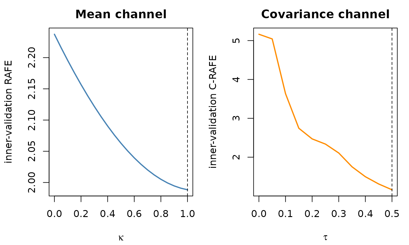
par(op)Does correcting the moments shrink the bound?
This is the question the package can answer directly, and it is worth asking before any portfolio is formed. We roll a 60-month training window, tune on it, and measure both channels against the realised moments of the following 60 months.
T_train <- 60L
T_eval  <- 60L
starts  <- seq(1L, nrow(R) - T_train - T_eval + 1L, by = 12L)

channels <- do.call(rbind, lapply(starts, function(s) {
  tr <- R[s:(s + T_train - 1L), ]
  ev <- R[(s + T_train):(s + T_train + T_eval - 1L), ]
  mu <- colMeans(ev); Sigma <- stats::cov(ev)
  fit <- sep_tune(tr, kappa_grid = kg, tau_grid = tg)
  data.frame(
    rafe_raw  = compute_rafe(colMeans(tr), mu, Sigma = Sigma),
    rafe_cor  = compute_rafe(fit$mu_tilde, mu, Sigma = Sigma),
    crafe_raw = compute_crafe(Sigma, stats::cov(tr)),
    crafe_cor = compute_crafe(Sigma, fit$Sigma_tilde),
    date      = ff12$date[s + T_train]
  )
}))

round(rbind(
  RAFE   = c(raw = median(channels$rafe_raw),  corrected = median(channels$rafe_cor),
             share_improved = mean(channels$rafe_cor  < channels$rafe_raw)),
  `C-RAFE` = c(raw = median(channels$crafe_raw), corrected = median(channels$crafe_cor),
             share_improved = mean(channels$crafe_cor < channels$crafe_raw))
), 3)
#>          raw corrected share_improved
#> RAFE   0.790     0.564          0.824
#> C-RAFE 4.351     1.396          1.000
Both channels fall. The covariance channel improves in every single window and its median drops by roughly a factor of three; the mean channel improves in about four windows out of five.
Not on average, but window by window:
op <- par(mfrow = c(2, 1), mar = c(3.2, 4.4, 2.2, 1))
matplot(channels$date, cbind(channels$crafe_raw, channels$crafe_cor),
        type = "l", lty = 1, lwd = 2, col = c("#9AA5B1", "#1f4e79"),
        xlab = "", ylab = "C-RAFE", main = "Covariance channel")
legend("topleft", c("uncorrected", "after sigma_crafe_floor()"), bty = "n",
       lwd = 2, col = c("#9AA5B1", "#1f4e79"))
matplot(channels$date, cbind(channels$rafe_raw, channels$rafe_cor),
        type = "l", lty = 1, lwd = 2, col = c("#9AA5B1", "#E8A33D"),
        xlab = "", ylab = "RAFE", main = "Mean channel")
legend("topleft", c("uncorrected", "after mu_rafe_stein()"), bty = "n",
       lwd = 2, col = c("#9AA5B1", "#E8A33D"))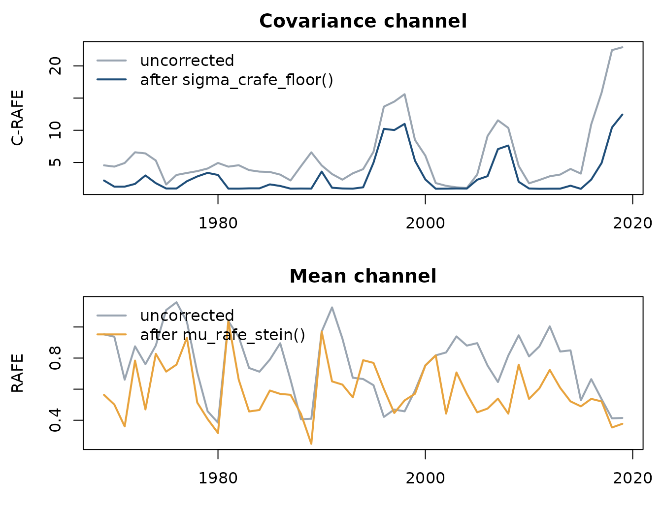
par(op)The covariance line never crosses: the floor helps in all 51 windows, and by the largest margin exactly when the uncorrected distortion spikes. The mean channel is noisier, which is what you would expect of a shrinkage estimator — it trades a small loss in calm periods for a large gain in turbulent ones.
Taking it to portfolios
T_hold <- 12L
tan_w  <- function(mu, S) { w <- drop(solve(S) %*% mu); w / sum(w) }

reb <- seq(1L, nrow(R) - T_train - T_hold + 1L, by = T_hold)
bt <- lapply(reb, function(s) {
  tr <- R[s:(s + T_train - 1L), ]
  ho <- R[(s + T_train):(s + T_train + T_hold - 1L), ]
  sp <- sep_tune(tr, kappa_grid = kg, tau_grid = tg)
  jt <- joint_trafe_tune(tr, kappa_grid = kg, tau_grid = tg)
  ws <- list(
    plugin = tan_w(colMeans(tr), stats::cov(tr)),
    sep    = tan_w(sp$mu_tilde, sp$Sigma_tilde),
    joint  = tan_w(jt$mu_tilde, jt$Sigma_tilde),
    `1/N`  = rep(1 / ncol(R), ncol(R))
  )
  list(r = vapply(ws, function(w) as.numeric(ho %*% w), numeric(T_hold)),
       pars = c(k_sep = sp$kappa, t_sep = sp$tau_rel,
                k_jnt = jt$kappa, t_jnt = jt$tau_rel))
})

rets <- do.call(rbind, lapply(bt, `[[`, "r"))
ann  <- function(x) c(mean = mean(x) * 12, sd = stats::sd(x) * sqrt(12),
                      sharpe = mean(x) / stats::sd(x) * sqrt(12))
round(t(apply(rets, 2, ann)), 3)
#>         mean    sd sharpe
#> plugin 0.208 2.284  0.091
#> sep    0.040 0.356  0.113
#> joint  0.040 0.356  0.113
#> 1/N    0.071 0.155  0.456
The uncorrected plug-in tangency portfolio is the disaster the literature leads you to expect: an annualised volatility above 200% and a Sharpe ratio near zero.
Correcting the moments cuts that volatility by about 85%, from roughly 2.28 to 0.36 annualised. The Sharpe ratio improves too, but far more modestly – from about 0.09 to 0.11 – because the correction shrinks the mean as well as the risk. Most of what the eigenvalue floor buys you here is the removal of enormous leveraged positions along badly-estimated directions, not extra return per unit of risk.
Plotted through time, the difference is not where you might expect it:
cum <- apply(rets, 2, cumsum)
dates_bt <- ff12$date[unlist(lapply(reb, function(s)
  (s + T_train):(s + T_train + T_hold - 1L)))]

matplot(dates_bt, cum, type = "l", lwd = 2, lty = c(1, 2, 1, 1),
        col = c("#B4413C", "#1f4e79", "#4FA3A5", "#E8A33D"),
        xlab = "", ylab = "cumulative monthly excess return",
        main = "Corrected vs uncorrected plug-in portfolios")
abline(h = 0, col = "grey60")
legend("topleft", colnames(rets), bty = "n", lwd = 2, lty = c(1, 2, 1, 1),
       col = c("#B4413C", "#1f4e79", "#4FA3A5", "#E8A33D"))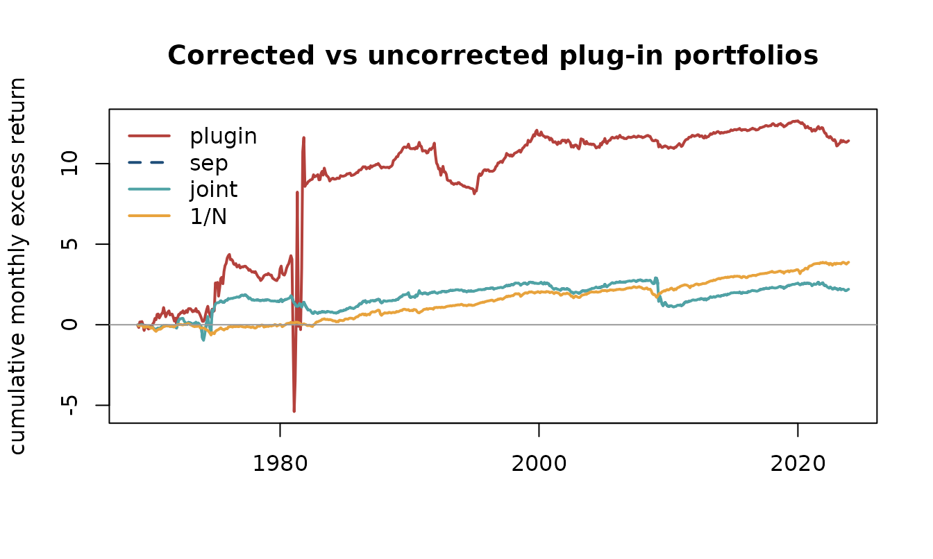
sep is drawn dashed because it lies exactly on top of
joint.
Read that chart carefully, because the naive reading is wrong. The uncorrected plug-in portfolio ends highest. Almost all of it comes from a single episode in 1981-82, visible as the near-vertical excursion: the strategy first loses several times its capital and then makes it back.
rbind(`worst monthly return` = round(apply(rets, 2, min), 3),
      `months below -100%`   = colSums(rets < -1),
      `cumulative sum`       = round(cum[nrow(cum), ], 2))
#>                      plugin    sep  joint    1/N
#> worst monthly return -8.332 -1.164 -1.164 -0.225
#> months below -100%    4.000  1.000  1.000  0.000
#> cumulative sum       11.420  2.200  2.200  3.880
A monthly return of is not a drawdown, it is ruin several times over: an investor holding that portfolio is wiped out and never reaches the recovery. The cumulative-sum convention above quietly assumes the position is refinanced at constant notional every month, which is what lets the red line come back at all. On a compounded basis the plug-in portfolio’s wealth goes negative and the path simply ends.
That is what the correction buys. It does not add return; it removes the leverage that makes the mean-variance solution uninvestable. The worst month falls from to , and the annualised volatility from 2.28 to 0.36.
And equal weighting still beats both, at about 0.46.
That is not a bug in the vignette, and it is worth stating plainly: on a
12-asset industry universe with unconstrained weights, 1/N
is a famously hard benchmark. The working paper’s claims rest on a
different and much more careful design – larger cross-sections,
non-overlapping inference, and comparison against Ledoit-Wolf and
nonlinear shrinkage rather than against a raw plug-in. Nothing here
reproduces them; see the paper.
The separability claim
The two tuners search different objectives, so there is no algebraic reason for them to agree. On this sample they do, in every rebalance:
pars <- do.call(rbind, lapply(bt, `[[`, "pars"))
c(kappa_agree = mean(pars[, "k_sep"] == pars[, "k_jnt"]),
  tau_agree   = mean(pars[, "t_sep"] == pars[, "t_jnt"]))
#> kappa_agree   tau_agree
#>           1           1

round(rbind(kappa = summary(pars[, "k_sep"]), tau = summary(pars[, "t_sep"])), 3)
#>       Min. 1st Qu. Median  Mean 3rd Qu. Max.
#> kappa  0.0   0.525    0.8 0.706     1.0  1.0
#> tau    0.1   0.250    0.5 0.397     0.5  0.5
That is the practical content of the separability claim: the bound’s
two channels can be tuned independently without loss, which turns a
two-dimensional grid search into two one-dimensional ones. If you are
tuning on a large cross-section, prefer sep_tune() — it is
the cheaper of the two and, here, selects identically.
One caveat on the grid. Relative floors are admitted on
[0, 0.5], which is the package default. On this universe
the selected
sits on the upper edge of that range in well over half the
rebalances:
c(tau_median = median(pars[, "t_sep"]),
  share_at_upper_edge = mean(pars[, "t_sep"] == max(tg)))
#>          tau_median share_at_upper_edge
#>              0.5000              0.5818
A boundary-binding parameter means the data wants more flooring than the grid allows, so the reported optimum is a constrained one. Widening the grid here does improve realised Sharpe — but it leaves the range the paper works in, so the package will not do it silently.